<?xml version="1.0" encoding="utf-8"?><feed xmlns="http://www.w3.org/2005/Atom" ><generator uri="https://jekyllrb.com/" version="3.10.0">Jekyll</generator><link href="https://kredd2506.github.io/Astro/Astro/feed.xml" rel="self" type="application/atom+xml" /><link href="https://kredd2506.github.io/Astro/Astro/" rel="alternate" type="text/html" /><updated>2026-06-10T05:53:42+00:00</updated><id>https://kredd2506.github.io/Astro/Astro/feed.xml</id><title type="html">ASTRA-sim · Collective Scaling</title><subtitle>Modeling AllReduce / AllGather scaling in ASTRA-sim across torus and switch topologies on the analytical and ns-3 backends — latency-bound vs bandwidth-bound as a function of message size and node count.
</subtitle><entry><title type="html">Validating with the ns-3 Packet-Level Backend</title><link href="https://kredd2506.github.io/Astro/Astro/2026/06/10/validating-with-ns3.html" rel="alternate" type="text/html" title="Validating with the ns-3 Packet-Level Backend" /><published>2026-06-10T00:00:00+00:00</published><updated>2026-06-10T00:00:00+00:00</updated><id>https://kredd2506.github.io/Astro/Astro/2026/06/10/validating-with-ns3</id><content type="html" xml:base="https://kredd2506.github.io/Astro/Astro/2026/06/10/validating-with-ns3.html"><![CDATA[<p>The <a href="https://kredd2506.github.io/Astro/2026/06/09/when-does-topology-matter.html">analytical results</a>
came from an idealized link model — fast, great for sweeping a 220-point grid,
but it does not model packet-level congestion, PFC, or congestion control.
ASTRA-sim’s <strong>ns-3 backend</strong> does. The question for this final post: do the
regimes survive once real protocol overhead is in the loop?</p>

<h3 id="the-setup">The setup</h3>

<p>I rebuilt the ns-3 backend (<code class="language-plaintext highlighter-rouge">./ns3 configure --enable-mpi &amp;&amp; ./ns3 build
AstraSimNetwork</code>) and ran a matched 8-node slice: a one-hop <strong>switch</strong> fabric vs
a <strong>ring</strong> (= 1-D torus), both pinned to <strong>400 Gbps / 500 ns</strong> links so the only
difference is fabric structure, driving the <em>same</em> Chakra workloads through
ns-3’s packet-level RDMA model across 16 KiB → 16 MiB.
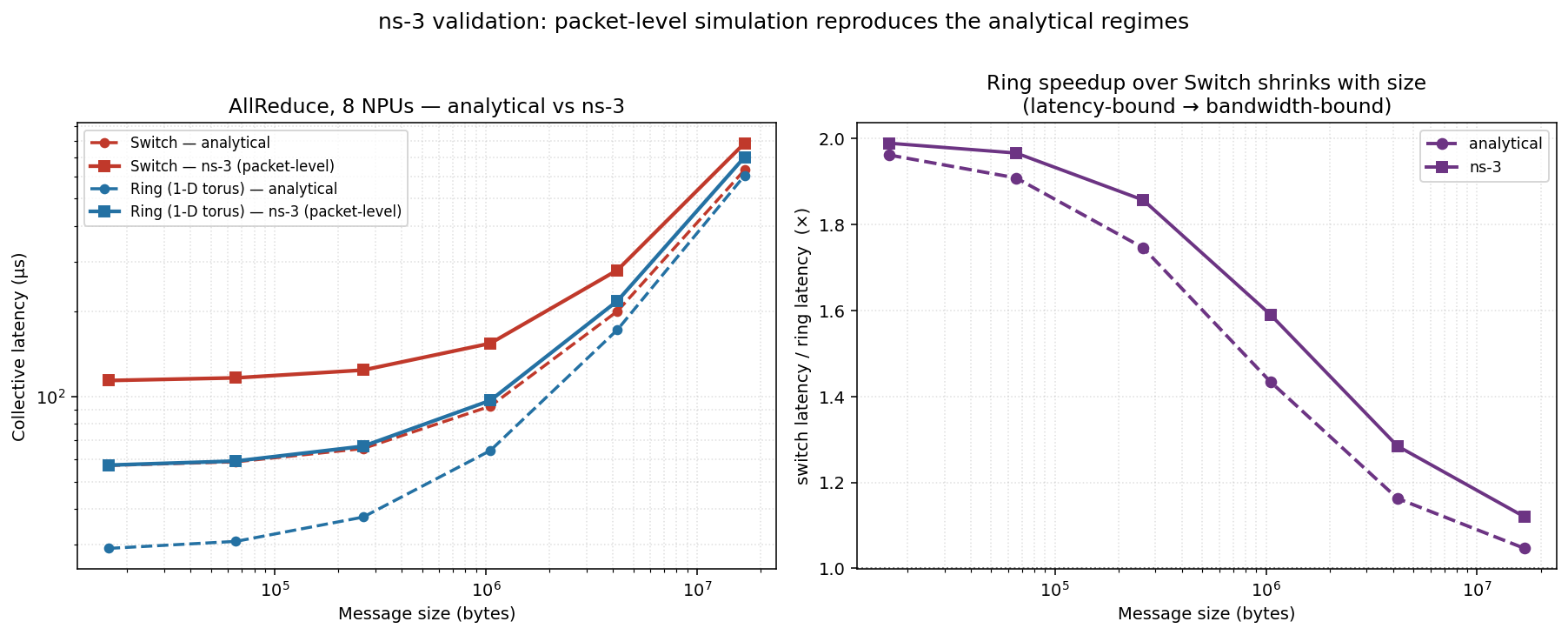
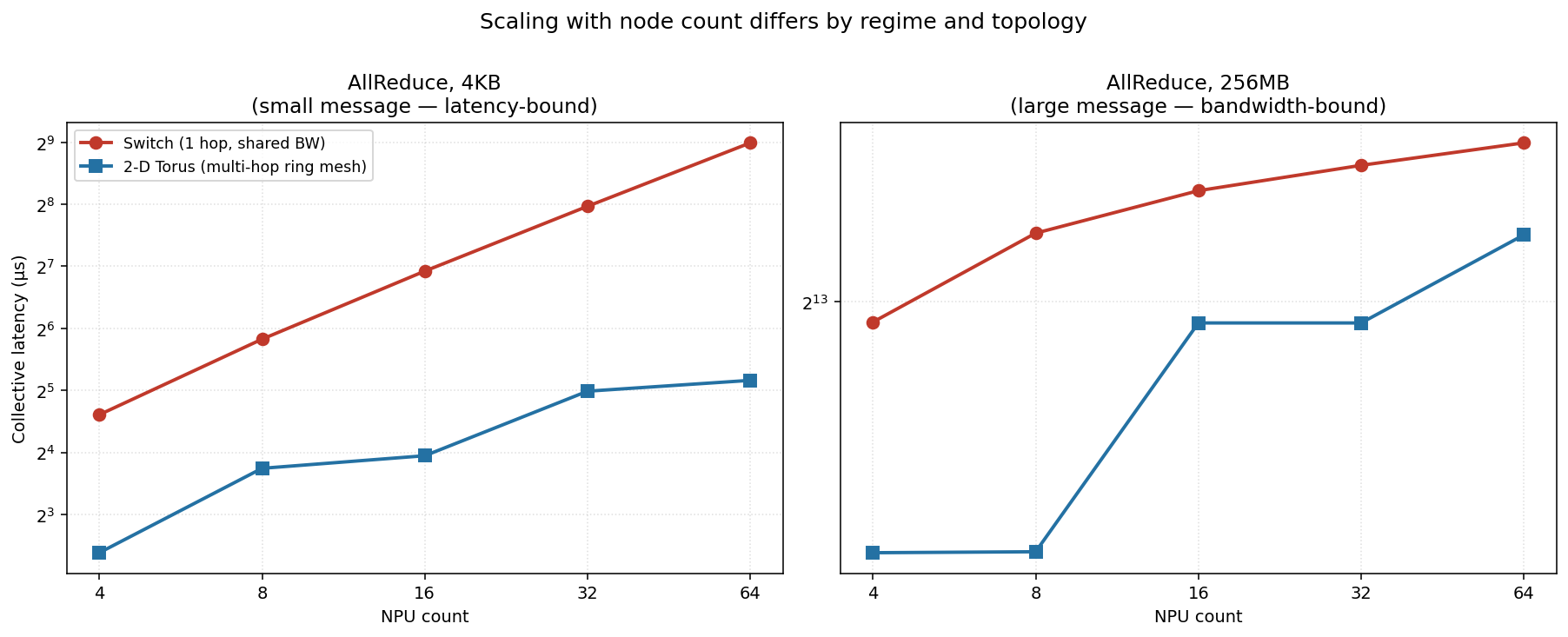
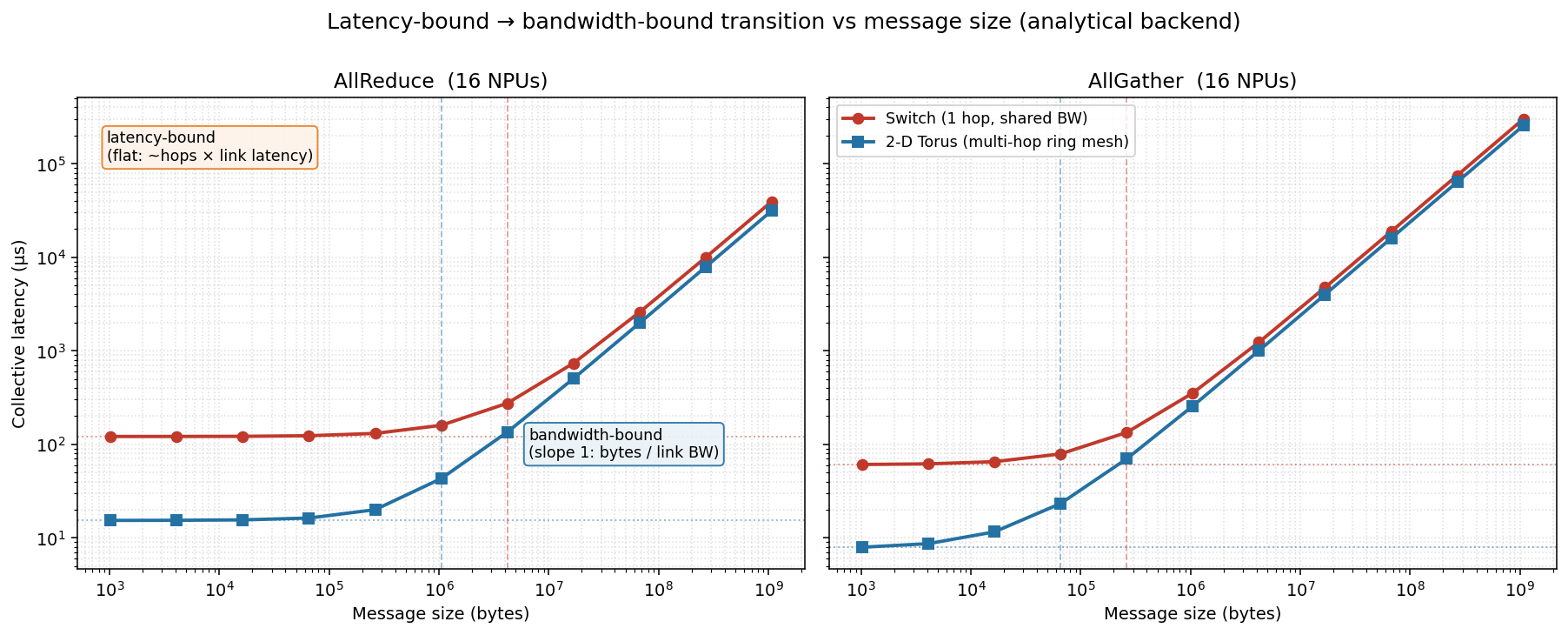
</p>

<p><img src="https://kredd2506.github.io/Astro/assets/astra/ns3_fig5_validation.png" alt="ns-3 vs analytical validation, 8 NPUs" /></p>

<h3 id="the-regimes-survive">The regimes survive</h3>

<p>ns-3 sits <strong>above</strong> the analytical model everywhere (left panel) — it pays for
packet headers and the congestion-control ramp the idealized model ignores, and
that overhead is <em>relatively</em> larger for small messages — but the <strong>shape is the
same</strong>: a flat latency-bound floor, a bandwidth-bound ramp, and ring
consistently below switch.
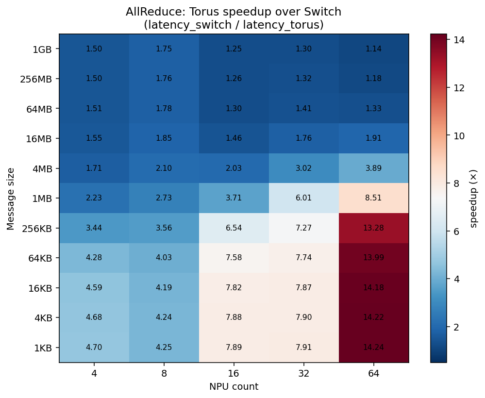
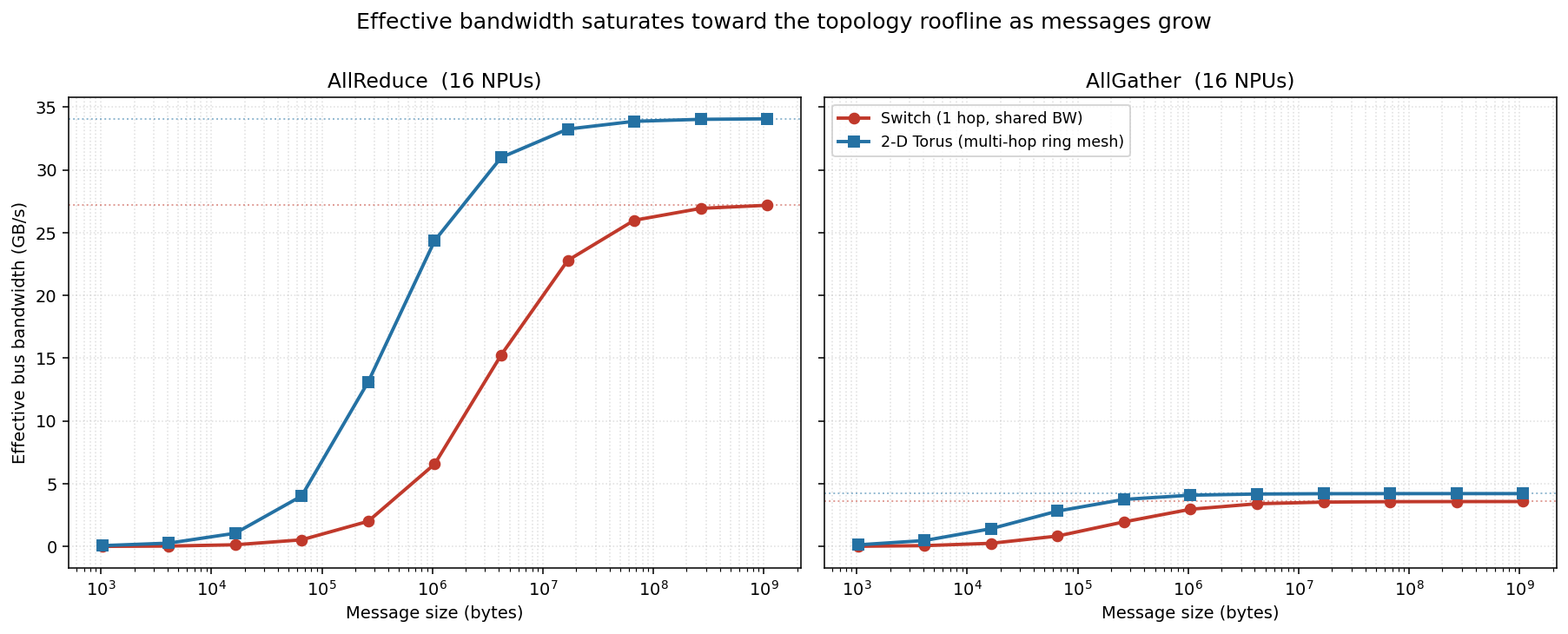
</p>

<p>The clincher is the right panel: the <strong>ring-over-switch speedup shrinks from ~2×
(latency-bound) toward ~1.1× (bandwidth-bound)</strong> in <em>both</em> backends, tracking
each other closely.</p>

<table>
  <thead>
    <tr>
      <th>Size</th>
      <th>switch (ns-3)</th>
      <th>ring (ns-3)</th>
      <th>speedup — ns-3 / analytical</th>
    </tr>
  </thead>
  <tbody>
    <tr>
      <td>16 KiB</td>
      <td>113.9 µs</td>
      <td>57.3 µs</td>
      <td><strong>1.99× / 1.96×</strong> (latency-bound)</td>
    </tr>
    <tr>
      <td>16 MiB</td>
      <td>784.6 µs</td>
      <td>700.7 µs</td>
      <td><strong>1.12× / 1.05×</strong> (bandwidth-bound)</td>
    </tr>
  </tbody>
</table>

<p>A second, more detailed simulator independently reproduces the central finding —
<strong>topology matters most when you’re latency-bound</strong> — which is exactly the
confidence cross-backend validation is supposed to buy.</p>

<h3 id="what-id-model-next">What I’d model next</h3>

<ul>
  <li><strong>3-D torus and fat-tree</strong> at 256–1024 NPUs, where diameter differences widen.</li>
  <li><strong>Algorithm × topology</strong>: halving-doubling and direct AllReduce, not just ring
— the latency floor is set by the algorithm’s step count, so the regime map
shifts.</li>
  <li><strong>ns-3 congestion at scale</strong>: where does PFC / back-pressure make the
analytical model optimistic?</li>
</ul>

<p>Code, configs, and all five figures:
<a href="https://github.com/kredd2506/Astro">github.com/kredd2506/Astro</a>.</p>]]></content><author><name></name></author><category term="astra-sim" /><category term="ns-3" /><category term="validation" /><category term="congestion" /><category term="results" /><summary type="html"><![CDATA[The analytical results came from an idealized link model — fast, great for sweeping a 220-point grid, but it does not model packet-level congestion, PFC, or congestion control. ASTRA-sim’s ns-3 backend does. The question for this final post: do the regimes survive once real protocol overhead is in the loop?]]></summary></entry><entry><title type="html">When Does Topology Matter? Scaling with Node Count</title><link href="https://kredd2506.github.io/Astro/Astro/2026/06/09/when-does-topology-matter.html" rel="alternate" type="text/html" title="When Does Topology Matter? Scaling with Node Count" /><published>2026-06-09T00:00:00+00:00</published><updated>2026-06-09T00:00:00+00:00</updated><id>https://kredd2506.github.io/Astro/Astro/2026/06/09/when-does-topology-matter</id><content type="html" xml:base="https://kredd2506.github.io/Astro/Astro/2026/06/09/when-does-topology-matter.html"><![CDATA[<p>The <a href="https://kredd2506.github.io/Astro/2026/06/08/latency-bound-vs-bandwidth-bound.html">previous post</a>
fixed the node count and swept message size. Here I do the opposite — fix the
message size and sweep the <strong>node count</strong> — because that’s where the two regimes
diverge most, and where topology choice either pays off enormously or barely
matters.</p>

<h3 id="scaling-with-node-count-depends-on-the-regime">Scaling with node count depends on the regime</h3>

<p><img src="https://kredd2506.github.io/Astro/assets/astra/analytical_fig3_scaling_vs_nodes.png" alt="Latency vs node count, small vs large message" /></p>

<p>This is the part that bites in practice. <strong>Latency-bound (left, 4 KB):</strong> the
switch’s latency grows almost <strong>linearly with N</strong> — 24 → 57 → 121 → 251 → 509 µs
from 4 to 64 NPUs — because ring-on-switch executes <code class="language-plaintext highlighter-rouge">N−1</code> sequential hops. The
torus grows far more slowly (steps scale with the longest dimension, ~<code class="language-plaintext highlighter-rouge">√N</code>).
<strong>Bandwidth-bound (right, 256 MB):</strong> both fabrics flatten out — adding nodes
barely changes time, because the per-node data volume of a ring collective is
nearly independent of <code class="language-plaintext highlighter-rouge">N</code> — and the gap narrows to a constant factor.</p>

<h3 id="one-picture-when-does-topology-matter">One picture: when does topology matter?</h3>

<p><img src="https://kredd2506.github.io/Astro/assets/astra/analytical_fig4_torus_speedup.png" alt="Torus speedup over switch across the size x node grid" /></p>

<p>Torus speedup over switch for AllReduce across every (size, node) cell. The story
is a <strong>gradient</strong>:</p>

<ul>
  <li><strong>Top-left (large messages):</strong> ~1.1–1.8×. Bandwidth-bound — topology is a
second-order effect; you’re paying for bytes either way.</li>
  <li><strong>Bottom-right (small messages, many nodes):</strong> up to <strong>14.2×</strong>. Latency-bound
at scale — topology is <em>everything</em>, because hop count is what you’re paying
for, and that’s exactly where torus and switch differ most (<code class="language-plaintext highlighter-rouge">N−1</code> sequential
switch hops vs ~<code class="language-plaintext highlighter-rouge">2(√N−1)</code> on the torus).</li>
</ul>

<p><strong>The takeaway for system design:</strong> if your collectives are small and frequent
(latency-bound — small gradients, frequent syncs, large clusters), fabric
topology dominates and a low-diameter mesh pays off enormously. If they’re large
and infrequent (bandwidth-bound — big tensors), you are buying raw link
bandwidth and the topology choice matters far less.</p>

<p>The analytical backend is an idealized link model, though. The
<a href="https://kredd2506.github.io/Astro/2026/06/10/validating-with-ns3.html">final post</a> checks these
regimes against ASTRA-sim’s <strong>ns-3</strong> packet-level backend.</p>]]></content><author><name></name></author><category term="astra-sim" /><category term="scaling" /><category term="topology" /><category term="torus" /><category term="switch" /><category term="results" /><summary type="html"><![CDATA[The previous post fixed the node count and swept message size. Here I do the opposite — fix the message size and sweep the node count — because that’s where the two regimes diverge most, and where topology choice either pays off enormously or barely matters.]]></summary></entry><entry><title type="html">Latency-Bound vs Bandwidth-Bound: The Two Regimes</title><link href="https://kredd2506.github.io/Astro/Astro/2026/06/08/latency-bound-vs-bandwidth-bound.html" rel="alternate" type="text/html" title="Latency-Bound vs Bandwidth-Bound: The Two Regimes" /><published>2026-06-08T00:00:00+00:00</published><updated>2026-06-08T00:00:00+00:00</updated><id>https://kredd2506.github.io/Astro/Astro/2026/06/08/latency-bound-vs-bandwidth-bound</id><content type="html" xml:base="https://kredd2506.github.io/Astro/Astro/2026/06/08/latency-bound-vs-bandwidth-bound.html"><![CDATA[<p>In the <a href="https://kredd2506.github.io/Astro/2026/06/07/modeling-collective-scaling-in-astra-sim.html">overview</a>
I set up a sweep of <code class="language-plaintext highlighter-rouge">AllReduce</code> / <code class="language-plaintext highlighter-rouge">AllGather</code> across a switch and a 2-D torus,
holding per-link physics identical. Here’s the first result: every collective
lives in one of two regimes, and the message size decides which.</p>

<h3 id="the-two-regimes-and-where-torus-separates-from-switch">The two regimes, and where torus separates from switch</h3>

<p><img src="https://kredd2506.github.io/Astro/assets/astra/analytical_fig1_latency_vs_size_16npus.png" alt="Latency vs message size, AllReduce and AllGather, 16 NPUs" /></p>

<p>Read each curve left to right. On the left, latency is <strong>flat</strong> — doubling a
tiny message barely moves it, because time is dominated by the fixed per-step
link latency, not the payload. This is the <strong>latency-bound</strong> regime. On the
right, every curve becomes a <strong>straight slope-1 line</strong> on log-log axes: latency
is now proportional to bytes, i.e. <strong>bandwidth-bound</strong>.</p>

<p>The two topologies sit on top of each other while latency-bound (same number of
algorithm steps), then the <strong>torus pulls clearly below the switch</strong> as messages
grow — its 2 links/node give more aggregate bandwidth than the switch’s shared
fabric. At 16 NPUs, AllReduce crosses from latency- to bandwidth-bound around
<strong>~1 MB on the torus</strong> but only around <strong>~4 MB on the switch</strong>: the switch’s
higher latency floor keeps it latency-bound longer.</p>

<h3 id="the-same-data-as-effective-bandwidth">The same data as effective bandwidth</h3>

<p><img src="https://kredd2506.github.io/Astro/assets/astra/analytical_fig2_effbw_vs_size_16npus.png" alt="Effective bus bandwidth vs message size, 16 NPUs" /></p>

<p>Plotting <em>delivered</em> bandwidth (bytes ÷ time) makes the transition tangible.
Small messages <strong>waste</strong> the fabric — almost all the time is latency, so
effective bandwidth is near zero. As messages grow, each curve climbs and
<strong>saturates toward a topology-dependent roofline</strong>. The torus’s roofline is
higher; the switch saturates lower. The knee of this curve <em>is</em> the
latency→bandwidth crossover from the first figure.</p>

<p>The practical reading: there is a minimum message size below which you simply
cannot use your fabric efficiently, and that threshold is <strong>higher on the
switch</strong>. If your collectives are smaller than the knee, you’re paying for
latency and buying more bandwidth won’t help.</p>

<p>Next: what happens as you scale the <strong>node count</strong> — where the two regimes
diverge most, and a single picture of when topology actually matters.</p>]]></content><author><name></name></author><category term="astra-sim" /><category term="allreduce" /><category term="allgather" /><category term="roofline" /><category term="results" /><summary type="html"><![CDATA[In the overview I set up a sweep of AllReduce / AllGather across a switch and a 2-D torus, holding per-link physics identical. Here’s the first result: every collective lives in one of two regimes, and the message size decides which.]]></summary></entry><entry><title type="html">Modeling Collective-Communication Scaling in ASTRA-sim</title><link href="https://kredd2506.github.io/Astro/Astro/2026/06/07/modeling-collective-scaling-in-astra-sim.html" rel="alternate" type="text/html" title="Modeling Collective-Communication Scaling in ASTRA-sim" /><published>2026-06-07T00:00:00+00:00</published><updated>2026-06-07T00:00:00+00:00</updated><id>https://kredd2506.github.io/Astro/Astro/2026/06/07/modeling-collective-scaling-in-astra-sim</id><content type="html" xml:base="https://kredd2506.github.io/Astro/Astro/2026/06/07/modeling-collective-scaling-in-astra-sim.html"><![CDATA[<p>When you train a large model across many accelerators, a surprising fraction of
wall-clock time is <em>not</em> spent doing math — it is spent in <strong>collective
communication</strong>: <code class="language-plaintext highlighter-rouge">AllReduce</code> to average gradients, <code class="language-plaintext highlighter-rouge">AllGather</code> to assemble
sharded tensors. How long those collectives take depends on three things that
interact in non-obvious ways: the <strong>message size</strong>, the <strong>number of nodes</strong>, and
the <strong>interconnect topology</strong>.</p>

<p>This is the first in a short series modeling that interaction directly in
<a href="https://github.com/astra-sim/astra-sim">ASTRA-sim</a> — Georgia Tech and Intel’s
distributed-ML network simulator. The question: <em>as message size and node count
vary, when is a collective <strong>latency-bound</strong> versus <strong>bandwidth-bound</strong>, and how
does that boundary move between a multi-hop <strong>torus</strong> and a one-hop <strong>switch</strong>
fabric?</em></p>

<h3 id="tldr-for-the-series">TL;DR for the series</h3>

<ul>
  <li>I swept <strong>AllReduce</strong> and <strong>AllGather</strong> over <strong>5 node counts (4–64)</strong> × <strong>11
message sizes (1 KiB–1 GiB)</strong> × <strong>2 topologies</strong> on ASTRA-sim’s analytical
backend (220 runs), holding per-link bandwidth (50 GB/s) and latency (500 ns)
identical so the <em>only</em> variable is fabric structure.</li>
  <li>Every curve shows the same two regimes: a <strong>flat latency-bound floor</strong> for
small messages (time ≈ algorithm steps × per-link latency) and a <strong>slope-1
bandwidth-bound ramp</strong> for large messages (time ≈ bytes ÷ link bandwidth).</li>
  <li><strong>The torus’s advantage is a strong function of regime</strong> — up to <strong>14×</strong>
latency-bound at scale, collapsing to <strong>~1.1–1.5×</strong> bandwidth-bound. (<a href="https://kredd2506.github.io/Astro/2026/06/08/latency-bound-vs-bandwidth-bound.html">the
full size sweep</a>,
<a href="https://kredd2506.github.io/Astro/2026/06/09/when-does-topology-matter.html">scaling with nodes</a>)</li>
  <li>An <strong>ns-3 packet-level</strong> run independently reproduces those regimes. (<a href="https://kredd2506.github.io/Astro/2026/06/10/validating-with-ns3.html">ns-3
validation</a>)</li>
</ul>

<h3 id="why-astra-sim-makes-this-clean">Why ASTRA-sim makes this clean</h3>

<p>ASTRA-sim separates three concerns, which is exactly what lets us isolate
topology:</p>

<table>
  <thead>
    <tr>
      <th>Layer</th>
      <th>What it specifies</th>
      <th>How I varied it</th>
    </tr>
  </thead>
  <tbody>
    <tr>
      <td><strong>Workload</strong></td>
      <td>the collective + message size (Chakra execution trace)</td>
      <td>synthetic single-op <code class="language-plaintext highlighter-rouge">AllReduce</code>/<code class="language-plaintext highlighter-rouge">AllGather</code> traces, <strong>1 KiB → 1 GiB</strong></td>
    </tr>
    <tr>
      <td><strong>System</strong></td>
      <td>the collective <em>algorithm</em> (ring, etc.)</td>
      <td>ring per dimension</td>
    </tr>
    <tr>
      <td><strong>Network</strong></td>
      <td>the <em>topology</em> + per-link BW/latency</td>
      <td><strong>switch</strong> (1 dim) vs <strong>2-D torus</strong> (Ring×Ring)</td>
    </tr>
  </tbody>
</table>

<p><strong>Topologies, held to identical link physics (50 GB/s, 500 ns):</strong></p>

<div class="language-yaml highlighter-rouge"><div class="highlight"><pre class="highlight"><code><span class="c1"># switch (one hop, bandwidth shared across the collective)</span>
<span class="na">topology</span><span class="pi">:</span>   <span class="pi">[</span> <span class="nv">Switch</span> <span class="pi">]</span>
<span class="na">npus_count</span><span class="pi">:</span> <span class="pi">[</span> <span class="nv">16</span> <span class="pi">]</span>
<span class="na">bandwidth</span><span class="pi">:</span>  <span class="pi">[</span> <span class="nv">50.0</span> <span class="pi">]</span>   <span class="c1"># GB/s</span>
<span class="na">latency</span><span class="pi">:</span>    <span class="pi">[</span> <span class="nv">500.0</span> <span class="pi">]</span>  <span class="c1"># ns</span>

<span class="c1"># 2-D torus (a multi-hop ring mesh; here 4x4 = 16 NPUs)</span>
<span class="na">topology</span><span class="pi">:</span>   <span class="pi">[</span> <span class="nv">Ring</span><span class="pi">,</span> <span class="nv">Ring</span> <span class="pi">]</span>
<span class="na">npus_count</span><span class="pi">:</span> <span class="pi">[</span> <span class="nv">4</span><span class="pi">,</span> <span class="nv">4</span> <span class="pi">]</span>
<span class="na">bandwidth</span><span class="pi">:</span>  <span class="pi">[</span> <span class="nv">50.0</span><span class="pi">,</span> <span class="nv">50.0</span> <span class="pi">]</span>
<span class="na">latency</span><span class="pi">:</span>    <span class="pi">[</span> <span class="nv">500.0</span><span class="pi">,</span> <span class="nv">500.0</span> <span class="pi">]</span>
</code></pre></div></div>

<p>The stock workload generator only takes integer <strong>MB</strong>, which can’t reach the
small-message latency-bound regime, so I wrote a <strong>bytes-based</strong> Chakra generator
to sweep cleanly on a log scale from 1 KiB. The analytical runs use the
<strong>congestion-unaware</strong> backend — the model built for multi-dimensional
(hierarchical) topologies — so the <em>same</em> backend drives both fabrics. Collective
latency is the <strong>max</strong> <code class="language-plaintext highlighter-rouge">sys[i] finished</code> cycle across ranks (the collective
finishes when the slowest rank does).</p>

<p>Everything is reproducible from a single Docker image; the harness lives at
<a href="https://github.com/kredd2506/Astro">github.com/kredd2506/Astro</a>. The next post
gets into the first result: the two regimes, and where torus separates from
switch.</p>]]></content><author><name></name></author><category term="astra-sim" /><category term="distributed-ml" /><category term="collectives" /><category term="overview" /><summary type="html"><![CDATA[When you train a large model across many accelerators, a surprising fraction of wall-clock time is not spent doing math — it is spent in collective communication: AllReduce to average gradients, AllGather to assemble sharded tensors. How long those collectives take depends on three things that interact in non-obvious ways: the message size, the number of nodes, and the interconnect topology.]]></summary></entry></feed>